梯度下降法的三种形式BGD、SGD以及MBGD对比

前面文章中，详细介绍了用批量梯度下降法（BGD），求解线性回归问题的过程。本文再另外介绍两种：随机梯度下降（SGD）和小批量梯度下降（MBGD），并使用图形的方式，对三种方法做一个横向对比。

import numpy as np

X = np.linspace(-1, 1, 100)
y = 5 * X  # 精简目标函数

def func(x, a):
    return a * x

# learning rate
lr = 0.05

批量梯度下降（Batch Gradient Descent BGD）

批量梯度下降，会遍历全部数据集算一次损失函数，然后算函数对各个参数的梯度，更新梯度。这种方法每更新一次参数，都要把数据集里的所有样本计算一遍，计算量大，计算速度慢。

a_bgd = 0
a_bgd_list = []

for step in range(200):
    a_sum = 0
    for idx, x in enumerate(X):
        a_sum += (func(x, a_bgd) - y[idx]) * x
    a_bgd -= lr * a_sum / len(X)
    a_bgd_list.append(a_bgd)

随机梯度下降（Stochastic Gradient Descent SGD）

随机梯度下降，是每次从训练集中随机选择一个样本，计算其对应的损失和梯度，进行参数更新，反复迭代。

这种方式在数据规模比较大时可以减少计算复杂度，从概率意义上来说的单个样本的梯度，是对整个数据集合梯度的无偏估计，但是它存在着一定的不确定性，因此收敛速率比批梯度下降得更慢。

a_sgd = 0
a_sgd_list = []

for step in range(200):
    idx = np.random.randint(len(X))
    x = X[idx]
    a_sum = (func(x, a_sgd) - y[idx]) * x
    a_sgd -= lr * a_sum
    a_sgd_list.append(a_sgd)

小批量梯度下降（Mini-batch Gradient Descent）

为了克服上面两种方法的缺点，采用的一种折中手段：将数据分为若干批次，按批次更新参数，每一批次中的一组数据共同决定了本次梯度的方向，下降起来就不容易跑偏，减少了随机性，另一方面，因为批的样本数比整个数据集少了很多，计算量也不是很大。

a_mbgd = 0
a_mbgd_list = []

for step in range(200):
    a_sum = 0
    idx = np.random.randint(len(X) - 10)
    for i in range(10):
        x = X[idx + i]
        a_sum += (func(x, a_mbgd) - y[idx + i]) * x
    a_mbgd -= lr * a_sum
    a_mbgd_list.append(a_mbgd)

对比和总结

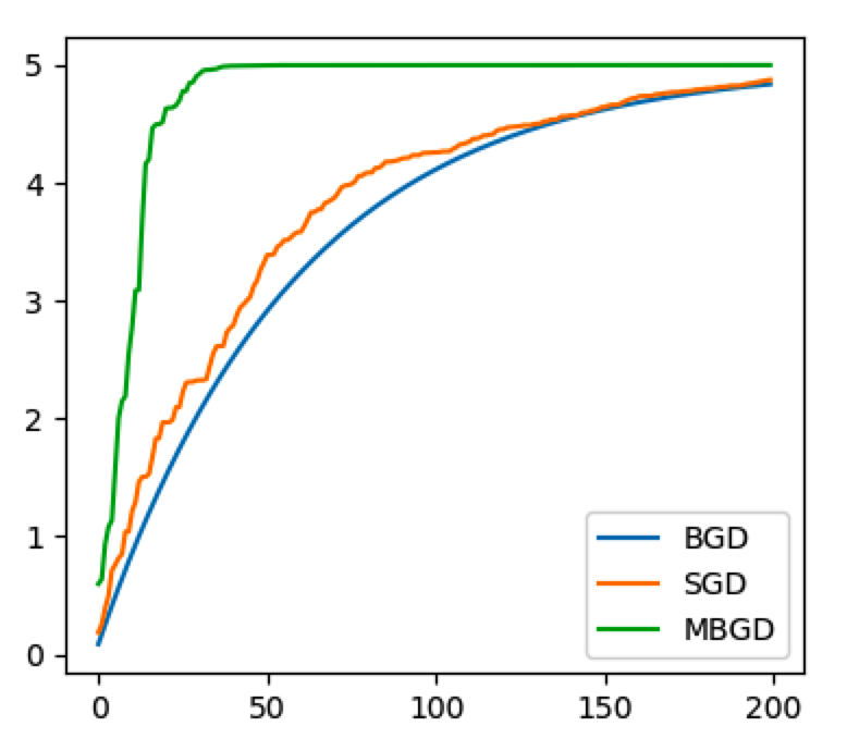
from matplotlib import pyplot as plt

plt.plot(range(200), a_bgd_list, label='BGD')
plt.plot(range(200), a_sgd_list, label='SGD')
plt.plot(range(200), a_mbgd_list, label='MBGD')
plt.legend() 
plt.show()

三种方法比较

1) SGD和BGD的迭代次数，要大于MBGD；

2) BGD一定能够得到一个局部最优解，SGD由于随机性的存在可能导致最终结果比BGD的差；

3) SGD有可能跳出某些小的局部最优解，所以一般情况下不会比BGD坏。

在实际项目中，一般优先使用SGD。